hydro emissions ms [ms]

INTRODUCTION

Hydroelectric dams are commonly believed to have no serious impact on the greenhouse effect, in contrast to fossil fuel use. However, the principal reason for this frequent assumption is ignorance of emissions of hydroelectric dams. Reservoirs in the Brazilian Amazonia (Legal Amazon) contribute to greenhouse gas emissions from the region, although contributions from currently existing reservoirs are small relative to other anthropogenic sources such as deforestation for cattle pasture. The four existing 'large' [> 10 megawatt (MW)] dams in the region are Balbina in the State of Amazonas (filled in 1987), Curuá-Una in Pará (1977), Samuel in Rondônia (1988) and Tucuruí in Pará (1984) (Figure 1). In addition, there are small reservoirs at Boa Esperança in Maranhão (filled prior to 1989), Jatapu in Roraima (1994), Paredão or Coarcy Nunes in Amapá (1975), and Pitinga in Amazonas (1982).

The scale of hydroelectric development contemplated for Amazonia makes this a potentially significant source of emissions of greenhouse gases in the future. Existing and planned dams are shown in Figure 2 and listed in Table I. Brazil's financial difficulties have repeatedly forced the national power authority (ELETROBRÁS) and the power monopoly in northern Brazil (ELETRONORTE) to postpone dam building plans. However, the overall scale of the plans, as distinguished from the expected date of completion of each dam, remains unchanged and consequently an important consideration for the future.

(Figures 1 and 2 and Table I here)

Little basis exists for calculating emissions from reservoirs. However, existing information can be organized in such a way as to draw the best possible conclusions given the limitations of our knowledge. The present paper assesses the amounts, types, and vertical distribution of biomass in areas flooded by reservoirs. Rough inferences are drawn as to emissions resulting from decay of this biomass, but the certainty that can be attached to them is low due to poor understanding of the rates and pathways of decay for flooded biomass. Hydroelectric emissions are the least well-understood of greenhouse gas emissions from Amazonian deforestation (hydroelectric flooding is considered to be a form of deforestation (cf. Fearnside, 1993).

The ultimate contribution of hydroelectric flooding to atmospheric carbon is much easier to calculate than the impact of this flooding on the annual balance of emissions, which requires knowledge of the rates of decay and of the proportions of carbon emitted as carbon dioxide (CO₂) and methane (CH₄); the latter of these is much more effective than the former in greenhouse warming per unit of weight. The ultimate contribution of dams to carbon emissions is the difference between the carbon stock in the forest prior to flooding and that in the reservoir once the forest has decayed and an equilibrium is reached. Reservoirs in tropical forest areas have a much greater potential for greenhouse gas emissions than do reservoirs in low biomass landscapes that characterize most of the world's existing hydroelectric dams. The amount of power generated also strongly affects the comparative impacts of hydroelectric versus fossil fuel generation.

In Amazonia, dams are frequently worse than petroleum from the point of view of the ultimate total of greenhouse gas emissions. The worst case is the Balbina Dam. Junk & Nunes de Mello (1987) calculated that it would take 114 years of fossil fuel burning to equal the carbon emissions of the forest flooded in Balbina. The calculation made by these authors considered Balbina's installed capacity of 250 megawatts (MW) and an area of 1650 km².

The installed capacity of a dam represents what would be generated if all turbines were to operate year-round. Because the flow of the Uatumã River at Balbina is only sufficient to run all turbines for a fraction of the year, output at the dam averages 112 MW, and losses in transmission to Manaus reduce the average delivered to 109 MW (Brazil, ELETRONORTE/MONASA/ENGE-RIO, 1976). The area of the reservoir used by Junk & Nunes de Mello (1987) was apparently chosen from preliminary estimates that foresaw an area considerably smaller than do more recent estimates. Considering the average power delivered to Manaus and the 'official' reservoir area of 2360 km² at the normal maximum operating level of 50-m elevation above mean sea level, Fearnside (1989) amended to 250 years Junk & Nunes de Mello's estimate of the time that petroleum would need to be burned to equal Balbina's ultimate emissions of carbon.

While useful as an illustration, calculation of the ultimate contribution to carbon emissions tells us little about the contribution to the annual balance of emissions. The United Nations Framework Convention on Climate Change (UN-FCCC), signed at the United Nations Conference on Environment and Development (UNCED) in Rio de Janeiro in June 1992 by 155 countries plus the European Union, stipulates that each nation must make an inventory of carbon stocks and fluxes of greenhouse gases. This implies that the annual balance of greenhouse gas fluxes will be the criterion adopted for assigning responsibility among nations for global warming. Because forest biomass in Amazonian reservoirs decays exceedingly slowly, the contribution to the annual balance is very different from the ultimate potential for emitting carbon.

In addition to the timing of emissions, the amount that is emitted as methane rather than carbon dioxide strongly influences the global warming impact of reservoirs. Per ton of carbon, methane is much more potent than carbon dioxide in provoking the greenhouse effect. The average lifetime of methane in the atmosphere is much shorter than that of carbon dioxide: 10.5 years versus 120 years, given a constant composition atmosphere as assumed by the Intergovernmental Panel for Climate Change (IPCC) (Isaksen et al., 1992: 56). Different methods of calculating global warming equivalence of the various greenhouse gases result in widely varying values for the importance of methane; those methods that consider indirect effects and those that give emphasis to impacts in the near future assign substantially more weight to methane.

The IPCC's preferred method of calculation in its 1992 Supplementary Report considers a 100-year time horizon without discounting and only considers direct effects (Isaksen et al., 1992: 56). This assigns each ton of methane gas a weight 11 times greater than each ton of carbon dioxide. If indirect effects are considered using the same time horizon, as was done in the IPCC's 1990 report (Shine et al., 1990: 60), the weight given to methane relative to CO₂ (the global warming potential) is 21. Because much of methane's global warming impact is through indirect effects, the current state of disagreement over an appropriate global warming potential for methane is likely to be resolved in favor of higher values, thereby increasing the relative importance of impacts from Amazonian hydroelectric reservoirs.

The Amazonian várzea (white water floodplain) has been identified as one of the world's major sources of atmospheric methane (Mooney et al., 1987). The várzea occupies about 2% of the 5 X 10⁶ km² Legal Amazon, the same percentage that would be flooded if all of the 100,000 km² of reservoirs planned for the region are created (Brazil, ELETROBRÁS, 1987: 150). Virtually all planned hydroelectric dams are in the forested portion of the region, of which they would represent approximately 2.5-2.9%. Were these reservoirs to contribute an output of methane per km² on the same order as that produced by the várzea, they would together represent a significant contribution to the greenhouse effect. This methane source would be a virtually permanent addition to greenhouse gas fluxes, rather than a one-time input like the CO₂ releases from forest decay.

AN APPROACH TO CALCULATING EMISSIONS FROM RESERVOIRS

In order to calculate emissions from hydroelectric reservoirs one must know the amounts of biomass present and the likely paths by which it will decay. The trees left standing in the reservoir are obviously an important component. The portion of the tree projecting out of the water can be assumed to decay through processes similar to those affecting trees in clearings for agriculture and ranching, with part of the biomass being ingested by termites (which emit a small amount of methane), and part decomposing through other forms of decay which, in the aerobic environment above the water, produce only CO₂. The biomass above the water level eventually falls into the water, thereby being transferred to the anoxic environments where decay is much slower--but also more likely to yield methane. The leaves and vines fall off the trees very quickly, and the branches and trunks fall at a much slower rate.

The reservoir can be divided into different zones, where aerobic and anoxic conditions will have different relative importance (Fig. 3). Part of the reservoir is alternately exposed and flooded as water levels fluctuate between the minimum and maximum normal operating levels. All biomass components in this zone, including litter and below-ground biomass, will be exposed to aerobic conditions at some time during the year. The portion of standing trunks in the permanently flooded zone that are located between the minimum and maximum normal operating levels will also be exposed to aerobic conditions.

(Figure 3 here)

For underwater biomass, a part of the biomass near the surface will be in an environment that has some oxygen. The anoxic zone does not correspond directly to the hypolimnion, and for purposes of decay is even closer to the water surface. At Balbina, for example, although a very small amount of oxygen is measurable as deep as 5-m (G. V. Peña, personal communication, 1993), persons interested in commercial exploitation of flooded timber consider any wood below 1-m to be unaffected by decay (E. V. C. Monteiro de Paula, personal communication, 1993).

Decay in the anoxic water zone is exceedingly slow, even for leaves that are generally believed to decay rapidly. ELETRONORTE commissioned the Delft Hydraulics Laboratory in Delft, The Netherlands, to produce a model for water quality in Balbina, (Brazil, ELETRONORTE, 1987: 261). The model, known as OXY-STRATIF, assumes that all leaves, litter and fine branches will decay within ten years. However, over five years after filling Balbina, much of this material is still present (although no quantitative information is available). The very slow nature of decay in the anoxic zone is illustrated by bundles of leaves that were placed at 5-m depth for studies of insects and other organisms in Balbina: after ten months the visual appearance of the leaves remained as green as the day when they were placed in the water. No macroscopic organisms colonized the leaves, and not even the slime that typically forms on decaying material was present (G. V. Peña, personal communication, 1993).

In shallow areas of the reservoirs, methane bubbling is easily observed. At both Balbina and Tucuruí, bubbles can be seen everywhere, even when no pressure is exerted, as by stepping on the bottom. The nature of the environment--devoid of oxygen, with relatively high temperatures and high levels of nutrients--makes it ideal for methane-producing decay processes.

Emissions from decaying forest biomass will be supplemented from decay of organic matter that enters the reservoir from rivers and streams that feed it, from soil organic matter, and from macrophytes that grow in the reservoir. The production of methane from these sources must be considered, although carbon dioxide need not be considered as a net addition (with the exception of any soil organic matter oxidized). Data on methane production from these sources, which may be loosely described as production from the water itself, are not available for any Amazonian reservoir, the closest available surrogate being natural lakes in the várzea.

Methane production from decomposition is not strictly identical to methane emission to the atmosphere, as some of the methane dissolved in the water column will instead by oxidized to CO₂ before entering the atmosphere. Because of the limited amount of mixing through the thermocline, high concentrations of methane in the water in the hypolimnion will only enter the atmosphere as the water passes through the turbines; at this point great quantities of methane can be expected to be released due to the abrupt reduction in pressure. This occurs, for example, in water passing through turbines in reservoirs in Canada (M. Lucotte, personal communication, 1993). However, not all methane will be exposed to the atmosphere in the reservoir and at the turbines, and some will occur downstream of the dam. The dissolved concentration of CH₄ in the water released from the turbines or over the spillway is an important measurement that needs to be made, but not all CH₄ present in these water flows can be considered as methane emissions--some CH₄ may be oxidized to CO₂ in the river (Rosa, 1992).

Methane-rich water from the hypolimnion is occasionally released in reservoirs in central and western Amazonia (Balbina and Samuel) when a cold wave (friagem) reduces surface temperature and causes dissolution of the thermocline (the barrier created by thermal stratification of the water column that prevents vertical mixing), resulting in a turnover in the water. Many fish die during these events, for example, in April 1993 at Balbina. These events are more frequent in the western part of Amazonia, and are not a factor in the eastern part of the region, where most planned reservoirs would be located.

GREENHOUSE GAS EMISSIONS

Parameters for Emissions Calculations

Estimating emissions from reservoirs first requires estimates of the area of forest flooded in each impoundment. The riverbed area within each reservoir must be estimated and subtracted from the water surface area. Riverbed areas are calculated in Table II from estimates of the length and average width of the rivers. The surface areas of the reservoirs were measured from LANDSAT-TM 1:250,000 scale images (Fearnside et al., nd). Previously deforested areas and riverbed areas are deducted when forest loss is calculated (Table III).

(Tables II and III here)

Vertical distribution of biomass, and classification into trunks, leaves and other components, is important for determining what portion of the biomass will decay above the water and what will decay underwater in the permanently flooded and seasonally flooded zones. The only existing biomass study that assigns the biomass to vertical strata is that of Klinge & Rodrigues (1973), done at INPA's Reserva Egler, 64 km east of Manaus. The approximate dry weights are given in Table IV. The forest at the Reserva Egler has a maximum height of 38.1 m, which must be assumed to apply to the forests in the four existing large reservoirs.

(Table IV here)

Biomass estimates specific for each reservoir are available for all except Curuá-Una (Table V). Fortunately, the forest flooded at Curuá-Una has an area of only 65 km², representing only 1.3% of the total 4824 km² of forest flooded by 1990 in the region (Table V). Biomass for Curuá-Una is assumed to be the average estimated for all areas deforested in the 1989-1990 period (Fearnside, nd-a). Based on the proportion in vertical strata (Table IV), the water depths at minimum and maximum operating levels (Table V), and the areas in each zone (Table V), the biomass is calculated for each reservoir in the following categories: above-water zone wood, surface water zone wood, anoxic water zone leaves and other non-wood (all assumed to fall to the bottom of the reservoir), and below-ground wood (Table V). The amounts of wood removed by logging prior to filling and after filling (through 1990) are also roughly estimated (Table V). After these calculations, the progression of biomass values is calculated for each year for each reservoir, zone and biomass component. This is done using rates of decay in each zone and rates of biomass falling from the above-water to the below-water zones; these rates and other parameters for emission calculations are given in Table VI. The resulting biomass distributions in 1990 are given in Table VII.

(Tables V, VI and VII here)

The decay rates for underwater biomass are known to be exceedingly slow, but actual measurements are completely lacking. The average lifetimes assumed here are: 50 years for wood in the surface water zone, 200 years for leaves in the anoxic water zone, 500 years for wood in the anoxic water zone, 500 years for below-ground biomass in the permanently flooded zone, and 50 years for below-ground biomass in the seasonally flooded zone (Table VI).

Methane is also produced from ongoing biological processes that are independent of the stock of original forest biomass. These include decomposition of organic matter entering the reservoir from the river, and from decay of macrophytes that grow on a portion of the reservoir surface. These rates are assumed to be equal to those that have been found for open water and for macrophyte beds in studies of natural várzea lakes (Table VIII). Only methane is considered from these sources, as the carbon dioxide that they also generate is recycled when the macrophytes and other plants regrow. Chemical characteristics of water in the Balbina reservoir, for example, (located on a black water river) differ in a number of ways from white water várzea lakes, making clear the importance of direct measurements of methane production in reservoirs.

(Table VIII here)

Simulation of Emissions over Time

The greenhouse gas fluxes by process in 1990 are presented in Table IX. While information on emissions from all sources at a given time, such as 1990, is needed as a baseline for assessing changes in greenhouse gas emissions, the evolution of emissions over time is important for evaluating potential impacts of planned projects. The timing of emissions is also very important in any system of emissions evaluation that gives differential weight to short-term and long-term impacts, as by discounting.

(Table IX here)

The emissions of CO₂ and CH₄ from Balbina are simulated for 50 years after closing in Figure 4. Methane emissions are fairly constant over the entire period, but carbon dioxide emissions are concentrated in a tremendous pulse in the first decade after closing. As of 1994, approximately half of the total CO₂ emission from Balbina had taken place, according to the simulation reported here.

(Figure 4 here)

The global warming impact of emissions can be converted to CO₂-equivalent carbon using global warming potentials adopted by the Intergovernmental Panel on Climate Change (IPCC) for direct effects only, over a 100-year time horizon without discounting (Isaksen et al., 1992). This is an underestimate of the true impact of reservoirs, as at least half of the global warming provoked by methane is through indirect rather than direct effects. In Figure 5 the CO₂-equivalent carbon of the emissions is simulated for 50 years for the four existing large reservoirs in Brazilian Amazonia.

(Figure 5 here)

Comparison with Fossil Fuel Emissions

Comparisons of emissions from hydroelectric projects with the avoided emissions from generating the same amount of power from fossil fuels are important because of the frequency with which hydroelectric projects have been promoted as offering a 'clean' alternative to thermoelectric generation. The examples of Balbina and Tucuruí are given in Table X. The mix of diesel and fuel oil burned at thermoelectric plants in Manaus (the city served by Balbina) is assumed to also apply to avoided emissions from Tucuruí. Emissions factors for these fuels applying to thermoelectric plants in Canada are assumed to apply to Brazil (probably an optimistic assumption). Power from Balbina substitutes for approximately 1.3 million t of CO₂-equivalent carbon (Table X, part F), far less than the emission of 6.9 million t from decaying biomass in the reservoir (Table XI). Table XI also compares 1990 emissions of Balbina and Tucuruí with emissions from other sources.

These Amazonian reservoirs compare poorly with two reservoirs in Canada that have been identified as sources of greenhouse gases (Rudd et al., 1993). The comparative impact of Balbina and Tucuruí is even worse than these emissions estimates indicate because the Canadian study used a global warming potential (GWP) for calculating the CO₂ equivalent of methane, which was over five times higher than the IPCC GWP used in the present paper. By converting emissions to CO₂ carbon equivalents using the same IPCC GWPs used in the current calculation, Rosa and Schaeffer (1994) have shown that the Canadian reservoirs studied by Rudd et al. (1993) have less global warming impact than would generating the same amount of energy from fossil fuel.

(Tables X and XI here)

In Figure 6 the emissions of Balbina are simulated over 50 years, in comparison to the emissions that would be produced by supplying the same energy to Manaus from fossil fuels. The tremendous disadvantage of hydroelectric generation in the initial years is evident. In the case of Balbina (which has a very large area per unit of electricity generated), even after 50 years (and probably for an indefinite period), the emissions will continue to exceed those from fossil fuels. These results call into question the image of Amazonian hydroelectric dams as helping to reduce global warming.

(Figure 6 here)

CONCLUSIONS

Hydroelectric reservoirs in Brazilian Amazonia emitted very approximately 0.26 million tons of CH₄ gas and 38 million tons of CO₂ gas in 1990. Of the CH₄, approximately 0.11 million tons were emitted from open water, 0.04 from macrophyte beds, < 0.01 from above-water decay of forest biomass, and 0.11 from underwater decay of forest biomass. The underwater decay rates are the least reliable of these estimates. No net carbon dioxide emissions come from open water or macrophytes. Above-water decay contributed approximately 99% of the estimated 38 million tons of CO₂ emitted. Using 1992 IPCC global warming potentials, these emissions are equivalent to approximately 11 million tons of CO₂-equivalent carbon.

The total area of planned reservoirs in Brazilian Amazonia is approximately 20 times the area present in 1990, implying a potential annual emission rate of about 5.2 million tons of methane. While the methane emission represents an essentially permanent addition to gas fluxes, the carbon dioxide is released in a tremendous pulse during the first decade after closure. These CO₂ emissions greatly exceed the avoided emissions from fossil fuel combustion.

ACKNOWLEDGMENTS

I thank Summer V. Wilson, Bruce R. Forsberg and Gladys V. Peña for comments on the manuscript.

SUMMARY

Existing hydroelectric dams in Brazilian Amazonia emitted about 0.26 million tons of methane and 38 million tons of carbon dioxide in 1990. The methane emissions represent an essentially permanent addition to gas fluxes from the region, rather than a one-time release. The total area of reservoirs planned in the region is about 20 times the area existing in 1990, implying a potential annual methane release of about 5.2 million tons. About 40% of this estimated release is from underwater decay of forest biomass, which is the most uncertain of the components in the calculation. Methane is also released in reservoirs from open water, macrophyte beds, and above-water decay of forest biomass.

Hydroelectric dams release a large pulse of carbon dioxide from above-water decay of trees left standing in the reservoirs, especially during the first decade after closing. This elevates the global warming impact of the dams to levels much higher than would occur by generating the same power from fossil fuels. In 1990, the impoundment behind the Balbina Dam (closed in 1987) had over 20 times more impact on global warming than would generating the same power from fossil fuels, while the Tucuruí Dam (closed in 1984) had 0.4 times the impact of fossil fuels. Because of the large area flooded per unit of electricity generated at Balbina, greenhouse gas emissions are expected to exceed avoided fossil fuel emissions indefinitely.

REFERENCES

ASELMANN, I. & CRUTZEN, P. J. (1990). A global inventory of wetland distribution and seasonality, net productivity, and estimated methane emissions. Pp. 441-9 in Soils and the Greenhouse Effect (Ed. A. F. Bouwman). Wiley, New York: 575 pp., illustr.

BARTLETT, K. B., CRILL, P. M., BONASSI, J. A., RICHEY, J. E. & HARRISS, R. C. (1990). Methane flux from the Amazon River floodplain: Emissions during rising water. J. Geophysical Research, 95 (D10), pp. 16,773-8.

BRAZIL, ELETROBRÁS. (1986). Plano de Recuperação Setorial. Ministério das Minas e Energia, Centrais Elétricas do Brasil (ELETROBRÁS), Brasília, Brazil.

BRAZIL, ELETROBRÁS. (1987). Plano 2010: Relatório Geral. Plano Nacional de Energia Elétrica 1987/2010. (dezembro de 1987). Ministério das Minas e Energia, Centrais Elétricas do Brasil (ELETROBRÁS), Brasília, Brazil: 269 pp.

BRAZIL, ELETRONORTE. (1985a). Aproveitamento Hidrelétrico de Balbina: Reservatório - N.A. 50 m. Centrais Elétricas do Norte do Brasil, S.A. (ELETRONORTE), Balbina, Amazonas, Brazil. Map scale: 1:100,000.

BRAZIL, ELETRONORTE. (1985b). UHE Balbina e Atendimento do Mercado Energético de Manaus. Junho/85. Relatório 26.657. Centrais Elétricas do Norte do Brasil, S.A. (ELETRONORTE), Brasília, Brazil.

BRAZIL, ELETRONORTE. (1985c). Políticas e Estratégias para Implementação de Vilas Residenciais. Centrais Elétricas do Norte do Brasil, S.A. (ELETRONORTE), Brasília, Brazil. Map.

BRAZIL, ELETRONORTE. (1987). Estudos Ambientais do Reservatório de Balbina. Relatório "Diagnóstico" BAL-50-1001-RE. Centrais Elétricas do Norte do Brasil, S.A. (ELETRONORTE), Brasília, Brazil: 308 pp.

BRAZIL, ELETRONORTE. (nd-a). Reservatório da UHE Samuel: Levantamento Planimêtrico. Centrais Elétricas do Norte do Brasil, S.A. (ELETRONORTE), Brasília, Brazil. Map scale: 1:40,000.

BRAZIL, ELETRONORTE. (nd-b). UHE Tucuruí: Plano de Utilização do Reservatório, Caracterização e Diagnóstico do Reservatório e de sua Área de Influência. TUC-10-263-46-RE Volume 1 - Texto. Centrais Elétricas do Norte do Brasil, S.A. (ELETRONORTE), Brasília, Brazil. Irregular pagination.

BRAZIL, ELETRONORTE. (nd [c. 1983]). Usina Hidrelétrica Tucuruí 8.000 MW. Centrais Elétricas do Norte do Brasil, S.A. (ELETRONORTE), Brasília, Brazil: 27 pp.

BRAZIL, ELETRONORTE. (nd [1987]). Livro Branco sobre o Meio Ambiente da Usina Hidrelétrica de Tucuruí. Centrais Elétricas do Norte do Brasil, S.A. (ELETRONORTE), Brasília, Brazil: 288 pp.

BRAZIL, ELETRONORTE. (nd [1992]a). Ambiente Desenvolvimento Tucuruí. Centrais Elétricas do Norte do Brasil, S.A. (ELETRONORTE), Brasília, Brazil: 32 pp.

BRAZIL, ELETRONORTE. (nd [1992]b). Ambiente Desenvolvimento Samuel. Centrais Elétricas do Norte do Brasil, S.A. (ELETRONORTE), Brasília, Brazil: 24 pp.

BRAZIL, ELETRONORTE/MONASA/ENGE-RIO. (1976). Estudos Amazônia, Relatório Final Volume IV: Aproveitamento Hidrelétrico do Rio Uatumã em Cachoeira Balbina, Estudos de Viabilidade. Centrais Elétricas do Norte do Brasil (ELETRONORTE)/MONASA Consultoria e Projetos Ltda./ENGE-RIO Engenharia e Consultoria, S.A., Brasília, Brazil. Irregular pagination.

BRAZIL, PROJETO RADAMBRASIL. (1981). Mosaico semi-controlado de Radar. Map Scale: 1:250,000. Folhas SA-22-ZC, SB-22-XA, SB-22-XB and SB-22-SD. Departamento Nacional de Produção Mineral (DNPM), Rio de Janeiro, Brazil.

DEVOL, A. H., RICHEY, J. H., FORSBERG, B. R. & MARTINELLI, L. A. (1990). Seasonal dynamics in methane emissions from the Amazon River floodplain to the troposphere. J. Geophysical Research, 95 (D10), pp. 16,417-26, 5 figs.

FEARNSIDE, P. M. (1989). Brazil's Balbina Dam: Environment versus the legacy of the pharaohs in Amazonia. Environmental Management, 13 (4), pp. 401-23, 5 figs.

FEARNSIDE, P.M. (1993). Deforestation in Brazilian Amazonia: The effect of population and land tenure. Ambio, 22(8), pp. 537-545, 4 figs.

FEARNSIDE, P. M. (nd-a). Biomass of Brazil's Amazonian forests. (In preparation).

FEARNSIDE, P. M. (nd-b). Amazonia and global warming: Annual balance of greenhouse gas emissions from land use change in Brazil's Amazon region. (In preparation).

FEARNSIDE, P. M., MEIRA FILHO, L. G. & TARDIN, A. T. (nd). Deforestation rate in Brazilian Amazonia. (In preparation).

FEARNSIDE, P. M., LEAL FILHO, N. & FERNANDES, P. M. (1993). Rainforest burning and the global carbon budget: Biomass, combustion efficiency and charcoal formation in the Brazilian Amazon. J. Geophysical Research, 98 (D9), pp. 16,733-43, 6 figs.

GOREAU, T. J. & MELLO, W. Z. (1987). Effects of deforestation on sources and sinks of atmospheric carbon dioxide, nitrous oxide, and methane from central Amazonian soils and biota during the dry season: A preliminary study. Pp. 51-66 in Proceedings of the Workshop on Biogeochemistry of Tropical Rain Forests: Problems for Research. (Ed. D. Athié, T.E. Lovejoy & P. de M. Oyens). Universidade de São Paulo, Centro de Energia Nuclear na Agricultura (CENA), Piracicaba, São Paulo, Brazil: 85 pp., illustr.

ISAKSEN, I. S. A., RAMASWAMY, V., RODHE, H. & WIGLEY, T. M. L. (1992). Radiative forcing of climate. Pp. 47-67 in Climate Change 1992: The Supplementary Report to the IPCC Scientific Assessment. (Ed. J. T. Houghton, B. A. Callander & S. K. Varney). Cambridge University Press, Cambridge, UK: 200 pp.

JAQUES, A. P. (1992). Canada's Greenhouse Gas Emissions: Estimates for 1990. Report EPS 5/AP/4. Environment Canada, Ottawa, Canada: 78 pp.

JUNK, W. J. & NUNES DE MELLO, J. A. (1987). Impactos ecológicos das represas hidrelétricas na bacia amazônica brasileira. Pp. 367‑85 in Homem e Natureza na Amazônia. (Ed. G. Kohlhepp & A. Schrader). Tübinger Geographische Studien 95 (Tübinger Beiträge zur Geographischen Lateinamerika-Forschung 3). Geographisches Institut, Universität Tübingen, Tübingen, Germany: iii + 507 pp., illustr.

JURAS, A. A. (1988). Progama de Estudos da Ictiofauna na Área de Atuação das Centrais Elétricas do Norte do Brasil, S.A. (ELETRONORTE). ELETRONORTE, Brasília, Brazil: 48 pp + annexes.

KLINGE, H. (1973). Biomasa y materia orgánica del suelo en el ecosistema de la pluviselva centro-amazónico. Acta Científica Venezolana, 24 (5), pp. 174-81.

KLINGE, H. & RODRIGUES, W. A. (1973). Biomass estimation in a central Amazonian rain forest. Acta Científica Venezolana, 24 (5), pp. 225-37.

KLINGE, H., RODRIGUES, W. A., BRUNIG, E. & FITTKAU, E. J. (1975). Biomass and structure in a Central Amazonian rain forest. Pp. 115‑22 in Tropical Ecological Systems: Trends in Terrestrial and Aquatic Research. (Ed. F. Golley & E. Medina). Springer-Verlag, New York: 398 pp., illustr.

MARTINELLI, L. A., VICTORIA, R. L., MOREIRA, M. Z., ARRUDA JR., G., BROWN, I. F., FERREIRA, C. A. C., COELHO, L. F., LIMA, R. P. & THOMAS, W. W. (1988). Implantação de parcelas para monitoreamento de dinâmica florestal na área de proteção ambiental, UHE Samuel, Rondônia: Relatório preliminar. Centro de Energia Nuclear na Agricultura (CENA), Piracicaba, São Paulo, Brazil. (Unpublished report: 72 pp).

MARTIUS, C., FEARNSIDE, P. M., WASSMANN, R. & BANDEIRA, A. G. (nd). Deforestation and methane release from termites in Amazonia. (In preparation).

MARTIUS, C., WASSMANN, R., THEIN, U., BANDEIRA, A.G., RENNENBERG, H., JUNK, W. & SEILER, W. (1993). Methane emission from wood-feeding termites in Amazonia. Chemosphere 26 (1-4), pp. 623-632.

MOONEY, H. A., VITOUSEK, P. M. & MATSON, P. A. (1987). Exchange of materials between terrestrial ecosystems and the atmosphere. Science, 238, pp. 926-32.

PAIVA, M. P. (1977). The Environmental Impact of Man‑Made Lakes in the Amazonian Region of Brazil. Centrais Elétricas Brasileiras, S.A. (ELETROBRÁS), Diretoria de Coordenação, Rio de Janeiro, Brazil: 69 pp.

REVILLA CARDENAS, J. D. (1986). Estudos de ecologia e controle ambiental na região do reservatório da UHE de Samuel. Convênio: ELN/MCT/CNPQ/INPA de 01.07.82. Relatório Setorial, Segmento: Estimativa da Fitomassa. Período julho-dezembro 1986. Instituto Nacional de Pesquisas da Amazônia (INPA), Manaus, Amazonas, Brazil: 194 pp.

REVILLA CARDENAS, J. D. (1987). Relatório: Levantamento e Análise da Fitomassa da UHE de Kararaô, Rio Xingú. Instituto Nacional de Pesquisas da Amazônia (INPA), Manaus, Amazonas, Brazil: 181 pp., illustr.

REVILLA CARDENAS, J. D. (1988). Relatório: Levantamento e Análise da Fitomassa da UHE de Babaquara, Rio Xingú. Instituto Nacional de Pesquisas da Amazônia (INPA), Manaus, Amazonas, Brazil: 277 pp., illustr.

REVILLA CARDENAS, J. D. & DO AMARAL, I. L. (1986). Estudos de Ecologia e Controle Ambiental na Região do Reservatório da UHE de Samuel: Convênio ELN/CNPq/INPA, de 01.07.82. Relatório Setorial, Segmento Minhocucus, Período janeiro/junho 1986. Instituto Nacional de Pesquisas da Amazônia (INPA), Manaus, Amazonas, Brazil: 5 pp.

REVILLA CARDENAS, J. D., KAHN, F. L. & GUILLAMET, J. L. (1982). Estimativa da fitomassa do reservatório da UHE de Tucuruí. Pp. 1-11 in Projeto Tucuruí, Relatório Semestral, Período janeiro/junho 1982, Vol. 2: Limnologia, Macrófitas, Fitomassa, Degradação da Fitomassa, Doenças Endêmicas, Solos. Brazil, Centrais Elétricas do Norte do Brasil, S.A. (ELETRONORTE) & Instituto Nacional de Pesquisas da Amazônia (INPA). INPA, Manaus, Amazonas, Brazil: 32 pp.

ROBERTSON, B.A. (1980). Composição, Abundância e Distribuição de Cladocera (Crustacea) na Região de Água Livre da Represa de Curuá‑Una, Pará. Masters Thesis, Fundação Universidade do Amazonas (FUA) & Instituto Nacional de Pesquisas da Amazônia (INPA). INPA, Manaus, Amazonas, Brazil: 105 pp.

ROSA, L.P. (1992). Untitled presentation at the INPE/OECD Workshop on Inventories of Net Anthropogenic Emissions of Greenhouse Gases, São José dos Campos, São Paulo, Brazil, 9-10 March 1992.

ROSA, L.P. & SCHAEFFER, R. (1994). Greenhouse gas emissions from hydroelectric reservoirs. Ambio 23(2), pp. 164-165.

RUDD, J. W. M., HARRIS, R., KELLY, C. A. & HECKY, R. E. (1993). Are hydroelectric reservoirs significant sources of greenhouse gases? Ambio, 22 (4), pp. 246-8, 1 fig.

SEVA, O. (1990). Works on the Great Bend of the Xingu--A Historic Trauma? Pp. 19-35 in Hydroelectric Dams on Brazil's Xingu River and Indigenous Peoples. (Ed. L. A. de O. Santos & L. M. M. de Andrade). Cultural Survival Report 30. Cultural Survival, Cambridge, Massachusetts, USA: 192 pp., illustr.

SHINE, K. P., DERWENT, R. G., WUEBBLES, D. J. & MORCRETTE, J-J. (1990). Radiative forcing of climate. Pp. 41-68 in Climate Change: The IPCC Scientific Assessment. (Ed. J. T. Houghton, G. J. Jenkins & J. J. Ephraums). Cambridge University Press, Cambridge, UK: 365 pp.

WASSMANN, R. & THEIN, U. G. (1989). Spatial and seasonal variation of methane emission from an Amazon floodplain lake. Paper presented at the Workshop on 'Cycling of Reduced Gases in the Hydrosphere,' SIL Congress, Munich, Germany, 17 August 1989. (Manuscript, 8 pp.)

FIGURE LEGENDS

Figure 1:Brazil's Legal Amazon region with the four existing large dams.

Figure 2:Seventy-nine planned and existing dams in Brazilian Amazonia. Only dams in the ELETRONORTE system are included, not those planed by State Governments or private firms. Redrawn from Seva (1990), who based the map on Brazil, ELETROBRÁS (1986) and Brazil, ELETRONORTE (1985c).

Figure 3:Zones for distribution of biomass in reservoirs.

Figure 4:Balbina: CO₂ and CH₄ emissions (million t of gas).

Figure 5:Hydroelectric greenhouse gas emissions (CO₂-equivalent carbon).

Figure 6:Balbina: Greenhouse gas emissions (CO₂-equivalent carbon).

TABLE I: EXISTING AND PLANNED DAMS IN BRAZILIAN AMAZONIA^a

Dam Dam name River Projected

No. Valley Installed

Capacity

(MW)

----------------------------------------------------------

1 São Gabriel Uaupés/Negro 2,000

2. Santa Isabel Uaupés/Negro 2,000

3. Caracaraí-Mucajaí Branco 1,000

4. Maracá Uraricoera 500

5. Surumu Cotingo 100

6. Bacarão Cotingo 200

7. Santo Antônio Cotingo 200

8. Endimari Ituxi 200

9. Madeira/Caripiana Mamoré/Madeira 3,800

10. Samuel Jamarí 200

11. Tabajara-JP-3 Ji-Paraná 400

12. Jaru-JP-16 Ji-Paraná 300

13. Ji-Paraná-JP-28 Ji-Paraná 100

14. Preto RV-6 Roosevelt 300

15. Muiraquitã RV-27 Roosevelt 200

16. Roosevelt RV-38 Roosevelt 100

17. Vila do Carmo AN-26 Aripuanã 700

18. Jacaretinga AN-18 Aripuanã 200

19. Aripuanã AN-26 Aripuanã 300

20. Umiris SR-6 Sucunduri 100

21. Itaituba Tapajós 13,000

22. Barra São Manuel Tapajós 6,000

23. Santo Augusto Juruena 2,000

24. Barra do Madeira Juruena 1,000

(Juruena)

25. Barra do Apiacás Teles Pires 2,000

26. Talama (Novo Horizonte) Teles Pires 1,000

27. Curuá-Una Curuá-Una 100

28. Belo Monte (Cararaô) Xingu 8,400

29. Babaquara Xingu 6,300

30. Ipixuna Xingu 2,300

31. Kokraimoro Xingu 1,900

32. Jarina Xingu 600

33. Iriri Iriri 900

34. Balbina Uatumã 300

35. Fumaça Uatumã 100

36. Onça Jatapu 300

37. Katuema Jatapu 300

38. Nhamundá/Mapuera Nhamundá 200

39. Cachoeira Porteira Trombetas 1,400

40. Tajá Trombetas 300

41. Maria José Trombetas 200

42. Treze Quedas Trombetas 200

43. Carona (Trombetas) 300

44. Carapanã Erepecuru 600

45. Mel Erepecuru 500

46. Armazém Erepecuru 400

47. Paciência Erepecuru 300

48. Curuá Curuá 100

49. Maecuru Maecuru 100

50. Paru III Paru 200

51. Paru II Paru 200

52. Paru I Paru 100

53. Jari IV Jari 300

54. Jari III Jari 500

55. Jari II Jari 200

56. Jari I Jari 100

57. F. Gomes Araguari 100

58. Paredão Araguari 200

59. Caldeirão Araguari 200

60. Arrependido Araguari 200

61. Santo Antônio Araguari 100

62. Tucuruí Tocantins 6,600

63. Marabá Tocantins 3,900

64. Santo Antônio Tocantins 1,400

65. Carolina Tocantins 1,200

66. Lajeado Tocantins 800

67. Ipueiras Tocantins 500

68. São Félix Tocantins 1,200

69. Sono II Sono 200

70. Sono I Sono 100

71. Balsas I Balsas 100

72. Itacaiúnas II Itacaiúnas 200

73. Itacaiúnas I Itacaiúnas 100

74. Santa Isabel Araguaia 2,200

75. Barra do Caiapó Araguaia 200

76. Torixoréu Araguaia 200

77. Barra do Peixe Araguaia 300

78. Couto de Magalhães Araguaia 200

79. Noidori Mortes 100

----------

Total: 85,900

----------------------------------------------------------------

a Based on list derived from ELETRONORTE sources by Seva (1990: 26-27). Dam numbers correspond to numbering in Figure 2.

TABLE II: RIVERBED AREAS IN AMAZONIAN RESERVOIRS

Reservoir River Length Average Riverbed Source

in width area

reservoir (m)^b (km²)

(km)^a

‑‑‑‑‑‑‑‑‑‑‑‑‑‑‑‑‑‑‑‑‑‑‑‑‑‑‑‑‑‑‑‑‑‑‑‑‑‑‑‑‑‑‑‑‑‑‑‑‑‑‑‑‑‑‑‑‑‑‑‑‑‑‑‑‑

Balbina Uatumã 210 139 29

Pitinga 100 99 10

Balbina total: 39^c

Curuá‑ Curuá-Una 80 69 6

Una Muju 40 35 1

Mojui dos Campos 20 15 0

Curuá-Una total: 7^d

Samuel Jamari 255 116 29^e

Tucuruí Tocantins 170 1891 321^f

TOTAL 397

‑‑‑‑‑‑‑‑‑‑‑‑‑‑‑‑‑‑‑‑‑‑‑‑‑‑‑‑‑‑‑‑‑‑‑‑‑‑‑‑‑‑‑‑‑‑‑‑‑‑‑‑‑‑‑‑‑‑‑‑‑‑‑‑

a Lengths of Balbina and Tucuruí from Juras (1988).

b River widths measured at approximately 5-km intervals using the following maps or images indicated under Source at the following scales: Balbina: 1:100,000; Samuel: 1:40,000; Tucuruí: 1:250,000. Widths of Curuá‑Una and tributaries are based on 6 direct measurements by Robertson (1980).

c Brazil, ELETRONORTE, 1985a.

d Robertson, 1980.

e Brazil, ELETRONORTE, nd-a.

f Brazil, Projeto RADAMBRASIL, 1981.

TABLE III: FLOODING BY HYDROELECTRIC DAMS

Dam State Dates of filling

‑‑‑‑‑‑‑‑‑‑‑‑‑‑‑‑‑‑‑‑‑‑‑‑‑‑‑‑‑‑‑‑‑‑‑‑‑‑‑‑‑‑‑‑‑‑‑‑‑‑‑‑‑------------

1 2 3

‑‑‑‑‑‑‑‑‑‑‑‑‑‑‑‑‑‑‑‑‑‑‑‑‑‑‑‑‑‑‑‑‑‑‑‑‑‑‑‑‑‑‑‑‑‑‑‑‑‑‑‑‑------------

Balbina Amazonas 1 Oct. 1987 ‑ 15 July 1989

Curuá‑Una Pará Jan. 1977 ‑ May 1977

Samuel Rondônia Oct. 1988‑ July 1989

Tucuruí Pará 6 Sept. 1984 ‑ 30 Mar. 1985

‑‑‑‑‑‑‑‑‑‑‑‑‑‑‑‑‑‑‑‑‑‑‑‑‑‑‑‑‑‑‑‑‑‑‑‑‑‑‑‑‑‑‑‑‑‑‑‑‑‑‑‑‑------------

TOTALS

‑‑‑‑‑‑‑‑‑‑‑‑‑‑‑‑‑‑‑‑‑‑‑‑‑‑‑‑‑‑‑‑‑‑‑‑‑‑‑‑‑‑‑‑‑‑‑‑‑‑‑‑‑------------

a Balbina riverbed area estimated from ELETRONORTE (1985a) 1:100,000 scale map; Curuá‑Una riverbed area calculated from map and river width measurements of Robertson (1980); Samuel riverbed area estimated from length; Tucuruí riverbed area from Brazil, Projeto RADAMBRASIL, 1981.

b Official areas for comparison only. Sources: Balbina: Brazil, ELETRONORTE, 1987; Curuá‑Una: Robertson, 1980: 9; Samuel: Revilla Cardenas, 1986; Tucuruí: Brazil, ELETRONORTE, nd [1987]: 24‑25.

c Three small dams outside the ELETRONORTE system are: Pitinga (filled in 1982 and raised in 1993; 1989 LANDSAT-measured area = 62 km²) near Balbina in Amazonas, Boa Esperança (filled prior to 1989; LANDSAT-measured area = 24 km²) in Maranhão, and Jatapu (filled in 1994; official area = 45 km²) in Roraima. All of the area flooded by these dams represents forest loss. The two dams filled prior to 1989 would bring the LANDSAT-measured total area to 6017 km² and the estimated forest loss to 5620 km².

d LANDSAT‑measured water surface includes riverbed and previous deforestation. To avoid double counting, estimated forest loss does not include previous deforestation: Column 8 = Column 7 ‑ Column 5. (Source: Fearnside et al., nd).

e Balbina 1988‑1989 rate is an overestimate due to lack of a 1988 image (230/61) covering approximately 10‑20% of the reservoir area nearest the dam. If unimaged area represented 10% of the measured 1988 area, then Balbina loss rate in 1988‑1989 was 348 km² yr^-1 (a decrease of 34%); if 20%, then loss rate was 162 km² yr^-1 (a 70% decrease).

f Area measured by Robertson (1980) from Centrais Elétricas do Para (CELPA) map. Paiva (1977) gives the official area as 86 km².

g Area cleared by ELETRONORTE only (Brazil, ELETRONORTE, nd[1987].

[Table III part 2]

Previous River‑ Official LANDSAT‑ Estimated 1988‑1989

defores‑ bed area measured forest forest

tation in area of water loss loss

flooded (km²)^a water surface (km²)^d rate

area surface area in (km² yr^-1)

(km²) (km²)^b 1989 (km²)^c

‑‑‑‑‑‑‑‑‑‑‑‑‑‑‑‑‑‑‑‑‑‑‑‑‑‑‑‑‑‑‑‑‑‑‑‑‑‑‑‑‑‑‑‑‑‑‑‑‑‑---------------

4 5 6 7 8 9

‑‑‑‑‑‑‑‑‑‑‑‑‑‑‑‑‑‑‑‑‑‑‑‑‑‑‑‑‑‑‑‑‑‑‑‑‑‑‑‑‑‑‑‑‑‑‑‑‑‑---------------

55 39 2,360 3,147 3,108 693^e

0 7 102 72 65^f 0

91 29 645 465 436 436

400^g 321 2,430 2,247 1,926 0

‑‑‑‑‑‑‑‑‑‑‑‑‑‑‑‑‑‑‑‑‑‑‑‑‑‑‑‑‑‑‑‑‑‑‑‑‑‑‑‑‑‑‑‑‑‑‑‑‑‑---------------

546 397 5,537 5,931 5,534 1,129

‑‑‑‑‑‑‑‑‑‑‑‑‑‑‑‑‑‑‑‑‑‑‑‑‑‑‑‑‑‑‑‑‑‑‑‑‑‑‑‑‑‑‑‑‑‑‑‑‑‑---------------

TABLE IV: BIOMASS BY STRATUM AT MANAUS: APPROXIMATE DRY WEIGHTS^a

Stratum Mean height Approximate dry weight biomass (t ha^-1)

(m)^b ‑‑‑‑‑‑‑‑‑‑‑‑‑‑‑‑‑‑‑‑‑‑‑---------------

-----‑‑‑‑‑‑‑‑‑‑‑‑‑‑‑‑ Leaves Stems Branches

Midpoint Range

(±)

‑‑‑‑‑‑‑‑‑‑‑‑‑‑‑‑‑‑‑‑‑‑‑‑‑‑‑‑‑‑‑‑‑‑‑‑‑‑‑‑‑‑‑‑‑‑‑‑‑‑---------------

A 29.6 5.9 1.1 66.1 23.1

B 21.1 4.4 3.4 127.9 58.5

C1 11.5 3.1 1.9 22.5 12.4

C2 4.8 1.2 1.0 4.8 1.7

D 2.4 0.7 1.0 0.9 0.3

E 0.6 0.5 0.3 0.4 0.0

‑‑‑‑‑‑‑‑‑‑‑‑‑‑‑‑‑‑‑‑‑‑‑‑‑‑‑‑‑‑‑‑‑‑‑‑‑‑‑‑‑‑‑‑‑‑‑‑‑----------------

8.6 222.5 96.0

‑‑‑‑‑‑‑‑‑‑‑‑‑‑‑‑‑‑‑‑‑‑‑‑‑‑‑‑‑‑‑‑‑‑‑‑‑‑‑‑‑‑‑‑‑‑‑‑‑‑---------------

Vines 21.9

Epiphytes 0.1

Totals for non-wood, 30.6

wood and all live

above-ground biomass

Fine litter^c 10.9

Downed dead wood^d

Standing dead wood^d

Totals for non-wood, 41.5

wood and all

above-ground biomass

‑‑‑‑‑‑‑‑‑‑‑‑‑‑‑‑‑‑‑‑‑‑‑‑‑‑‑‑‑‑‑‑‑‑‑‑‑‑‑‑‑‑‑‑‑‑‑‑‑‑---------------

a Data for fresh weights from Klinge & Rodrigues (1973), converted to dry weights using a constant correction factor of 0.475 derived for these data by the same authors (Klinge et al., 1975).

b Maximum height of the stand was 38.1 m. The stand is located 64 km east of Manaus at INPA's Reserva Egler.

c Average of 5 measurements at hydroelectric dam sites at Samuel, Belo Monte and Babaquara (Revilla Cardenas, 1987, 1988; Martinelli et al., 1988).

d Klinge, 1973: 179.

[Table IV, part 2]

Percent of total above-ground biomass

‑‑‑‑‑‑‑‑‑‑‑‑‑‑-- ‑‑‑‑‑‑‑‑‑‑‑‑‑‑‑‑‑‑‑‑‑‑‑‑‑‑‑‑‑‑‑‑‑‑‑‑‑----------

Total Total Leaves Stems Branches Total Total

live live live live

wood biomass wood biomass

‑‑‑‑‑‑‑‑‑‑‑‑‑‑-- ‑‑‑‑‑‑‑‑‑‑‑‑‑‑‑‑‑‑‑‑‑‑‑‑‑‑‑‑‑‑‑‑‑‑-------------

89.3 90.3 0.28 17.15 6.00 23.14 23.43

186.4 189.8 0.87 33.17 15.16 48.33 49.21

34.9 36.7 0.48 5.83 3.21 9.04 9.52

6.5 7.4 0.25 1.23 0.44 1.68 1.92

1.2 2.2 0.27 0.22 0.09 0.31 0.58

0.4 0.7 0.07 0.10 0.00 0.10 0.17

‑‑‑‑‑‑‑‑‑‑‑‑‑‑‑‑‑‑‑‑‑‑‑‑‑‑‑‑‑‑‑‑‑‑‑‑‑‑‑‑‑‑‑‑‑‑‑‑‑‑‑‑‑‑‑----------

318.5 327.1 2.23 57.69 24.91 82.60 84.83

‑‑‑‑‑‑‑‑‑‑‑‑‑‑‑‑‑‑‑‑‑‑‑‑‑‑‑‑‑‑‑‑‑‑‑‑‑‑‑‑‑‑‑‑‑‑‑‑‑‑‑‑‑‑‑‑‑‑‑‑‑----

5.67

0.03

318.5 349.1 7.92 82.60 90.52

2.83

18.02 4.67

7.6 1.97

344.2 385.6 10.76 89.24 100.00

‑‑‑‑‑‑‑‑‑‑‑‑‑‑‑‑‑‑‑‑‑‑‑‑‑‑‑‑‑‑‑‑‑‑‑‑‑‑‑‑‑‑‑‑‑‑‑‑‑‑‑‑‑‑‑‑---------

TABLE V: BIOMASS PRESENT AND DIVISION BY ZONES IN AMAZONIAN RESERVOIRS

Dam Year Water Forest Forest

filled surface flooded flooded

area at at oper- at

operating ating minimum

level level level

(ha) (ha) (ha)

‑‑‑‑‑‑‑‑‑‑‑‑‑‑‑‑‑‑‑‑‑‑‑‑‑‑‑‑‑‑‑‑‑‑‑‑‑‑‑‑‑‑‑‑‑-----

Balbina 1987 314,700 310,840 206,829

Curuá-Una 1977 7,200 6,480 5,500

Samuel 1988 46,500 43,551 30,901

Tucuruí 1984 224,700 192,553 106,787

‑‑‑‑‑‑‑‑‑‑‑‑‑‑‑‑‑‑‑‑‑‑‑‑‑‑‑‑‑‑‑‑‑‑‑‑‑‑‑‑‑‑‑‑‑‑‑‑‑‑

TOTALS 593,100 553,424 350,017

‑‑‑‑‑‑‑‑‑‑‑‑‑‑‑‑‑‑‑‑‑‑‑‑‑‑‑‑‑‑‑‑‑‑‑‑‑‑‑‑‑‑‑‑‑‑‑‑‑‑

a Brazil, ELETRONORTE, 1987; forest flooded at minimum level is adjusted by ratio of LANDSAT‑measured area to official area at the operating level.

b Paiva, 1977: 17 (value for average depth at maximum operating level).

c Revilla Cardenas & do Amaral, 1986; forest area flooded at minimum water level taken as proportional to water volumes at these two levels from Brazil, ELETRONORTE, nd [1992]b: 5.

d Revilla Cardenas et al., 1982.

e Uses 58.0 m above mean sea level as minimum normal operating level (Brazil, ELETRONORTE, nd [ca. 1983]. A minimum operating level of 51.6 m (Brazil, ELETRONORTE, nd‑b: p. 2‑1; Brazil ELETRONORTE, nd [1992]a) implies drawdown depth of only 3.3 m. Forest area flooded at minimum water level is taken as proportional to water volumes at these two levels from Brazil, ELETRONORTE, nd [ca. 1983], p. 6).

f Brazil, ELETRONORTE, nd [1992]a.

g Brazil, ELETRONORTE, nd [1992]b.

[Table V, part 2]

Approx- Above‑ Biomass Average Depth

imate ground source depth at source

total biomass minimum

biomass (t ha^-1) level

(t ha^-1) (m)

‑‑‑‑‑‑‑‑‑‑‑‑‑‑‑‑‑‑‑‑‑‑‑‑‑‑‑‑‑‑‑‑‑‑‑‑‑‑‑‑‑‑‑‑‑‑---------

441 336 a, pp. 6.2 a, p. 14

172-3

428 327 Fearnside, 6.2 b

nd-a

557 425 c, p. 4 5.3 b

517 394 d, p. 90 9.7 e

‑‑‑‑‑‑‑‑‑‑‑‑‑‑‑‑‑‑‑‑‑‑‑‑‑‑‑‑‑‑‑‑‑‑‑‑‑‑‑‑‑‑‑‑‑----------

‑‑‑‑‑‑‑‑‑---‑‑‑‑‑‑‑‑‑‑‑‑‑‑‑‑‑‑‑‑‑‑‑‑‑‑‑‑‑‑‑‑--‑--------

[Table V, part 3]

Dam Initial biomass by zone (t dry matter ha^-1)

--------‑‑‑‑‑‑‑‑‑‑‑‑‑‑‑‑‑‑‑‑‑‑‑‑‑‑‑‑‑‑‑‑‑‑‑‑‑‑‑‑‑‑‑‑‑‑‑‑‑‑‑‑‑‑--

Above- Surface Anoxic Anoxic Below- Total

water water water water ground

wood wood wood leaves wood

and other

non-wood

‑‑‑‑‑‑‑‑‑‑‑‑‑‑‑‑‑‑‑‑‑‑‑‑‑‑‑‑‑‑‑‑‑‑‑‑‑‑‑‑‑‑‑‑‑‑‑‑‑‑‑‑‑‑----------

Balbina 264.69 4.55 31.44 35.70 104.74 441.12

Curuá-Una 257.11 4.42 30.54 34.68 101.74 428.50

Samuel 339.59 5.74 34.56 45.11 132.34 557.34

Tucuruí 291.40 5.33 55.47 41.82 122.69 516.71

‑‑‑‑‑‑‑‑‑‑‑‑‑‑‑‑‑‑‑‑‑‑‑‑‑‑‑‑‑‑‑‑‑‑‑‑‑‑‑‑‑‑‑‑‑‑‑‑‑‑‑‑‑‑----------

[Table V, part 4]

Dam Logging removals Fraction Fraction Years of post-

of biomass of above- of original filling logging

(t ha^-1of ground anoxic activity

reservoir area) wood zone ‑‑‑---------------

‑‑‑‑‑‑‑‑‑‑‑‑‑‑‑-- removed wood Begin End

Before After before removed

filling filling filling after

filling

‑‑‑‑‑‑‑‑‑‑‑‑‑‑‑‑‑‑‑‑‑‑‑‑‑‑‑‑‑‑‑‑‑‑‑‑‑‑‑‑‑‑‑‑‑‑‑‑‑‑‑‑‑‑‑‑‑‑‑‑‑‑‑‑‑Balbina 0 0 0.5 1993 2000

Curuá-Una 0 0 0 0

Samuel 0.2 0

Tucuruí 0.01 0.5 1988 2000

‑‑‑‑‑‑‑‑‑‑‑‑‑‑‑‑‑‑‑‑‑‑‑‑‑‑‑‑‑‑‑‑‑‑‑‑‑‑‑‑‑‑‑‑‑‑‑‑‑‑‑‑‑‑‑‑‑‑‑‑‑‑‑‑‑

[Table V, part 5]

Area cleared prior Draw- Draw-

to filling (ha) down down

‑‑‑‑‑‑‑‑‑‑‑‑‑‑‑‑‑‑‑‑‑‑‑‑‑‑‑‑ depth depth

Season- Perma- Total (m) source

ally nently

flooded flooded

zone zone

‑‑‑‑‑‑‑‑‑‑‑‑‑‑‑‑‑‑‑‑‑‑‑‑‑‑‑‑‑‑‑‑‑‑‑‑‑‑‑‑‑‑‑‑‑

0 5,000 5,000 4

4.5 guess

7 f, p. 5

2,000 8,000 10,000 14 g, p. 5

‑‑‑‑‑‑‑‑‑‑‑‑‑‑‑‑‑‑‑‑‑‑‑‑‑‑‑‑‑‑‑‑‑‑‑‑‑‑‑‑‑‑‑‑‑

TABLE VI: PARAMETERS FOR HYDROELECTRIC DAM EMISSION CALCULATIONS

Parameter Value

‑‑‑‑‑‑‑‑‑‑‑‑‑‑‑‑‑‑‑‑‑‑‑‑‑‑‑‑‑‑‑‑‑‑‑‑‑‑‑‑‑‑‑‑‑‑-------------------

Above-ground fraction 0.773

Average depth of surface water zone 1

Leaf decay rate in seasonally inundated zone -0.5

Above-water decay rate (0-4 yrs) -0.1691

Above-water decay rate (5-7 yrs) -0.1841

Above-water decay rate (8-10 yrs) -0.0848

Above-water decay rate (>10 yrs) -0.0987

Fraction of above-water decay via termites 0.0844

Wood decay rate in surface water zone -0.0139

Leaf decay rate in anoxic water zone -0.0035

Wood decay rate in anoxic water zone -0.0014

Below-ground decay rate in permanently flooded zone -0.0014

Below-ground decay rate in seasonally flooded zone -0.0139

Fraction of C released as CH₄ in termite decay 0.002

Fraction of C released as CH₄ in termite decay (high 0.0079

trace gas scenario)

Fraction of C released as CH₄ in surface water zone decay 0

Fraction of C released as CH₄ in anoxic water zone decay 1

Fraction of C released as CH₄ in below-ground decay 1

Fraction of water covered by macrophytes 0.1

Methane release from macrophyte beds 174.67

Methane release from open water 53.93

Carbon content of wood 0.50

Carbon content of leaves and fine litter 0.45

Carbon content of vines and epiphytes 0.45

Rate of wood fall from above-water zone 0.1155

Fraction of CH₄ oxidized in water 0

Leaf aerobic decay, first year 0.025

Leaf aerobic decay, after first year 0.0085

‑‑‑‑‑‑‑‑‑‑‑‑‑‑‑‑‑‑‑‑‑‑‑‑‑‑‑‑‑‑‑‑‑‑‑‑‑‑‑‑‑‑‑‑‑‑‑------------------

Biomass of components in unlogged original forests

Average total biomass of forest 428

Average water depth at minimum level 10

Initial biomass present: leaves 7.30

Initial biomass present: fine litter 8.75

Initial biomass present: vines and epiphytes 18.64

Initial biomass present: wood above water 240.33

Initial biomass present: wood in surface zone 4.42

Initial biomass present: wood in anoxic zone 47.32

Initial biomass present: below-ground 101.74

[Table VI, part 2]

Units Source

‑‑‑‑‑‑‑‑‑‑‑‑ ‑‑‑‑‑‑‑‑‑‑‑‑‑‑‑‑‑‑‑‑‑‑‑‑‑‑‑‑‑‑‑‑‑‑‑‑‑‑‑‑‑‑‑‑‑‑‑‑‑--

Fearnside, nd-a

meter Assumption, based on commercial timber spoilage

Fraction yr^-1 Assumption

Fraction yr^-1Assumed same as felled forest (Fearnside, nd-b)

Fraction yr^-1 Assumed same as felled forest (Fearnside, nd-b)

Fraction Assumed same as felled forest (Martius et al., nd)

Fraction yr^-1 Assumption: average lifetime = 50 years

Fraction yr^-1 Assumption: average lifetime = 200 years

Fraction yr^-1 Assumption: average lifetime = 500 years

Fraction yr^-1 Assumption: average lifetime = 50 years

Calculated from measurement by Martius et al., 1993

for Nasutitermes macrocephalus (a várzea species)

Calculated from measurement by Martius et al., 1993

for Nasutitermes macrocephalus (a várzea species)

Assumption

µg m^-2 day^-1 Table VIII

Fearnside et al., 1993

Assumption

Fraction yr^-1 Assumption: average lifetime = 6 years

Assumption

Fraction of Calculated from Brazil, ELETRONORTE, 1987: 261

original (OXY-STRATIF model parameter for Balbina). Value

leaf biomass divided by 10 (as a guess at the exaggeration in

lost annually OXY-STRATIF)

Fraction of Calculated from Brazil, ELETRONORTE, 1987: 261.

original Value divided by 10 (as a guess at the exaggeration

leaf biomass in OXY-STRATIF)

lost annually

‑‑‑‑‑‑‑‑‑‑‑‑ -‑‑‑‑‑‑‑‑‑‑‑‑‑‑‑‑‑‑‑‑‑‑‑‑‑‑‑‑‑‑‑‑‑‑‑‑‑‑‑‑‑‑‑‑‑‑‑---

t ha^-1

meters Assumption

t ha^-1 Calculated from total biomass and Table IV.

TABLE VII: APPROXIMATE QUANTITIES OF BIOMASS PRESENT IN 1990

(10⁶ t of biomass)

PERMANENTLY FLOODED ZONE (at minimum operating water level)

Above- Surface Anoxic Anoxic

water water water water

wood wood wood leaves

and other

non-wood

‑‑‑‑‑‑‑‑‑‑‑‑‑‑‑‑‑‑‑‑‑‑‑‑‑‑‑‑‑‑‑‑‑‑‑‑‑‑‑‑-------------------------

Balbina 28.85 0.89 20.50 7.09

Curuá-Una 0.04 0.02 0.84 0.15

Samuel 6.17 0.11 2.17 1.07

Tucuruí 6.00 0.41 13.01 3.52

‑‑‑‑‑‑‑‑‑‑ ‑‑‑‑‑‑‑‑‑‑‑‑‑‑‑‑‑‑‑‑‑--------‑‑‑‑‑‑‑‑‑------

TOTALS 41.06 1.44 36.52 11.84

‑‑‑‑‑‑‑‑‑‑ ‑‑‑‑‑‑‑‑‑‑‑‑‑‑‑‑‑‑‑‑‑‑‑‑‑‑‑‑‑‑--------------

SEASONALLY FLOODED ZONE (at maximum normal operating water level)

Above- Leaves Under- Below-

water and water ground

wood other wood wood

non-wood

‑‑‑‑‑‑‑‑‑‑ ‑‑‑‑‑‑‑‑‑‑‑‑‑‑‑‑‑‑‑‑‑--------‑‑‑‑‑‑‑‑‑-------

Balbina 19.61 2.02 2.41 10.11

Curuá-Una 0.04 0.00 0.01 0.08

Samuel 2.77 0.42 0.46 1.57

Tucuruí 7.47 0.78 6.35 9.54

----------- -------‑‑‑‑‑‑‑‑‑‑‑‑‑‑‑‑‑‑‑‑‑‑‑‑‑‑‑‑‑‑‑‑‑-----

TOTALS 29.88 3.22 9.23 21.30

‑-‑‑‑‑‑---- -------‑‑‑‑‑‑‑‑‑‑‑‑‑‑‑‑‑‑‑‑‑‑‑‑‑‑------------

[Table VII, part 2]

Below- Total

ground

wood

‑‑‑‑‑‑‑‑‑‑‑‑‑‑‑‑

27.19 84.52

0.51 1.56

3.04 12.57

10.46 33.41

‑‑‑‑‑‑‑‑‑‑‑‑‑‑‑‑

41.20 132.05

‑‑‑‑‑‑‑‑‑‑‑‑‑‑‑‑

Total

‑‑‑‑‑‑‑‑

34.14

0.13

5.22

24.14

‑‑‑‑‑‑‑‑

63.64

‑‑‑‑‑‑‑‑

TABLE VIII: METHANE EMISSIONS FROM AMAZON FLOODPLAIN ECOSYSTEMS

Habitat Methane flux

(mg CH₄ m^-2 day^-1

‑‑‑‑‑‑‑‑‑‑‑‑‑‑‑‑‑‑‑‑‑‑‑‑‑ ‑‑‑‑‑‑‑‑‑‑‑‑‑‑‑‑‑‑‑‑‑‑‑‑‑‑‑‑‑‑‑‑‑‑‑

Low High Eight

water water lakes

CAMREX CAMREX near

cruise 11 cruise 9 Manaus

(1) (1) (1)

‑‑‑‑‑‑‑‑‑‑‑‑‑‑‑‑‑‑‑‑‑‑‑‑‑ ‑‑‑‑‑‑‑‑‑‑‑‑‑‑‑‑‑‑‑‑‑‑‑‑‑‑‑‑‑‑‑‑‑‑‑

Lakes, open water 40 88 58

(±12) (±30) (±16)

Lakes, macrophyte beds 131 390 251

(±47) (±109) (±58)

Lakes, flooded forest 7.1 74 55

(±3.4) (±19) (±13)

‑‑‑‑‑‑‑‑‑‑‑‑‑‑‑‑‑‑‑‑‑‑‑‑- ‑‑‑‑‑‑‑‑‑‑‑‑‑‑‑‑‑‑‑‑‑‑‑‑‑‑‑‑‑‑‑‑‑‑‑

Sources:

(1) Devol et al., 1990.

(2) Wassmann & Thein, 1989.

(3) Bartlett et al., 1990.

(4) For comparison, Aselmann & Crutzen (1990: 446) estimate the average for lakes of the world to be 43 mg CH₄ m^-2 day^-1.

[Table VIII, part 2]

‑‑‑‑‑‑‑‑------------------------------------------

Lago da Machantaria NASA/ Value

(near Manaus) ABLE assumed for

‑‑‑‑‑‑‑‑‑‑‑‑‑‑----------- rising Amazonian

Low Rising High water reservoirs

water water water

(2) (2) (2) (3) (4)

‑‑‑‑‑‑‑‑‑‑‑‑‑‑‑‑‑‑‑‑‑‑‑‑‑‑‑‑‑‑‑‑‑‑‑‑----

50-100 5-50 5-25 74 53.9

(±14)

dry 0-50 0-100 201 174.7

(±35)

dry 0‑200 0‑200 126

(±20)

‑‑‑‑‑‑‑‑‑‑‑‑‑‑‑‑‑‑‑‑‑‑‑‑‑‑‑‑‑‑‑‑‑‑‑‑----

TABLE IX: GREENHOUSE GAS FLUXES BY PROCESS IN 1990 FROM HYDROELECTRIC DAMS^a

PERMANENTLY INUNDATED ZONE

Area Above‑water decay Underwater decay

of ‑‑‑‑‑‑‑‑‑‑‑‑‑‑‑‑‑‑‑‑‑‑‑‑‑‑‑ ‑‑‑‑‑‑----------

perma- Termites Other Wood in surface

nently ‑‑‑‑‑‑‑‑‑‑‑‑‑‑‑‑‑‑ water zone

inunda- CH₄ CO₂ CO₂ ‑‑‑‑‑‑‑‑‑-------

ted zone (10⁶ (10⁶ (10⁶ CH₄

(ha) t gas) t gas) t gas) (10⁶

t gas)

‑‑‑‑‑‑‑‑‑‑‑‑‑‑‑‑‑‑‑‑ ‑‑‑‑‑‑‑‑‑‑‑‑‑‑‑‑‑‑‑‑‑‑‑‑‑‑‑ ‑‑‑‑------------

Balbina 206,829 0.00 0.28 8.61 0.00

Curuá-Una 5,500 0.00 0.00 0.01 0.00

Samuel 30,901 0.00 0.06 1.84 0.00

Tucuruí 106,787 0.00 0.06 1.98 0.00

‑‑‑‑‑‑‑‑‑‑‑‑‑‑‑‑‑‑‑‑ ‑‑‑‑‑‑‑‑‑‑‑‑‑‑‑‑‑‑‑‑‑‑‑‑‑‑‑‑‑ ‑‑‑‑----------

TOTALS 350,017 0.00 0.41 12.43 0.00

-------------------- ----------------------------- --------------

[Table IX, part 2]

Below-ground decay

‑‑‑‑‑‑‑‑‑‑‑‑‑‑‑‑‑‑‑‑‑‑‑‑‑‑‑‑‑‑‑‑‑‑‑‑‑‑‑‑‑‑‑‑-‑ ‑‑‑‑‑‑‑‑‑‑‑‑‑‑‑‑--

Wood in anoxic Leaves and other

water zone non-wood biomass

‑‑‑‑‑‑‑‑‑‑‑‑‑‑‑‑‑‑‑‑‑‑‑‑‑‑‑‑‑‑‑‑‑‑‑‑‑‑‑‑‑‑‑‑‑-- CH₄ CO₂

CO₂ CH₄ CO₂ CH₄ CO₂ (10⁶ (10⁶

(10⁶ (10⁶ (10⁶ (10⁶ (10⁶ t gas) t gas)

t gas) t gas) t gas) t gas) t gas)

‑‑‑‑‑‑‑‑‑‑‑‑‑‑‑‑‑‑‑‑‑‑‑‑‑‑‑‑‑‑‑‑‑‑‑‑‑‑‑‑‑‑‑‑‑‑ ‑‑‑‑‑‑‑‑‑‑‑‑‑‑‑--

0.02 0.02 0.00 0.01 0.10 0.03 0.00

0.00 0.00 0.00 0.00 0.00 0.00 0.00

0.00 0.00 0.00 0.00 0.05 0.00 0.00

0.01 0.01 0.00 0.01 0.05 0.01 0.00

‑‑‑‑‑‑‑‑‑‑‑‑‑‑‑‑‑‑‑‑‑‑‑‑‑‑‑‑‑‑‑‑‑‑‑‑‑‑‑‑‑‑‑‑‑‑ ‑‑‑‑‑‑‑‑‑‑‑‑‑‑----

0.04 0.03 0.00 0.02 0.20 0.04 0.00

---------------------------------------------- ------------------

[Table IX, part 3]

SEASONALLY INUNDATED ZONE

Area Above‑water decay

of ‑‑‑‑‑‑‑‑‑‑‑‑‑‑‑‑‑‑‑‑‑‑‑‑‑‑‑

season‑ Termites Other

ally ‑‑‑‑‑‑‑‑‑‑‑‑‑‑‑‑‑‑

inunda- CH₄ CO₂ CO₂

ted zone (10⁶ (10⁶ (10⁶

(ha) t gas) t gas) t gas)

‑‑‑‑‑‑‑‑‑‑‑‑‑‑‑‑‑‑‑ ‑‑‑‑‑‑‑‑‑‑‑‑‑‑‑‑‑‑‑‑‑‑‑‑‑‑-

Balbina 104,011 0.0004 0.46 14.22

Curuá-Una 980 0.0000 0.00 0.03

Samuel 12,650 0.0001 0.07 2.16

Tucuruí 85,766 0.0002 0.23 7.06

‑‑‑‑‑‑‑‑‑‑‑‑‑‑‑‑‑‑‑ ‑‑‑‑‑‑‑‑‑‑‑‑‑‑‑‑‑‑‑‑‑‑‑‑‑‑-

TOTALS 203,407 0.0006 0.77 23.47

‑‑‑‑‑‑‑‑‑‑‑‑‑‑‑‑‑‑‑ ‑‑‑‑‑‑‑‑‑‑‑‑‑‑‑‑‑‑‑‑‑‑‑‑‑‑-

[Table IX, part 4]

Underwater decay Below‑ground decay

‑‑‑‑‑‑‑‑‑‑‑‑‑‑‑‑‑‑‑‑‑-‑‑‑‑‑‑‑‑‑‑‑‑‑‑---

Wood Leaves and other ‑‑‑‑‑‑‑‑‑‑‑‑‑‑‑‑‑‑

non-wood biomass

‑‑‑‑‑‑‑‑‑‑‑‑‑‑‑‑‑‑‑‑‑-‑‑‑‑‑‑‑‑‑‑‑‑‑‑---- CH₄ CO₂

CH₄ CO₂ CH₄ CO₂ (10⁶ (10⁶

(10⁶ (10⁶ (10⁶ (10⁶ t gas) t gas)

t gas) t gas) t gas) t gas)

‑‑‑‑‑‑‑‑‑‑‑‑‑‑‑‑‑‑‑‑‑-‑‑‑‑‑‑‑‑‑‑‑‑‑‑‑‑‑‑ ‑‑‑‑‑‑‑‑‑‑‑------

0.002 0.000 0.005 0.05 0.00007 0.00

0.000 0.000 0.000 0.00 0.00000 0.00

0.000 0.000 0.001 0.02 0.00001 0.00

0.006 0.000 0.002 0.05 0.00006 0.00

‑‑‑‑‑‑‑‑‑‑‑‑‑‑‑‑‑‑‑‑‑-‑‑‑‑‑‑‑‑‑‑‑‑‑‑‑‑‑‑ ‑‑‑‑‑‑‑‑‑‑----‑‑‑

0.009 0.000 0.007 0.13 0.00014 0.00

‑‑‑‑‑‑‑‑‑‑‑‑‑‑‑‑‑‑‑‑‑-‑‑‑‑‑‑‑‑‑‑‑‑‑‑‑‑‑‑ ‑‑‑‑‑‑‑‑‑‑‑‑‑----

[Table IX, part 5]

ENTIRE RESERVOIR

Area of Open Macro- Total from above-

reser- water phyte water decay

voir beds ‑‑‑‑‑‑‑‑‑‑‑‑‑‑‑‑‑-----

at oper-

ating CH₄ CH₄ CH₄ CO₂

level (10⁶ (10⁶ (10⁶ (10⁶

(ha) t gas) t gas) t gas) t gas)

‑‑‑‑‑‑‑‑‑‑‑‑‑‑‑‑‑‑‑‑‑‑‑‑‑‑‑‑‑‑‑‑‑‑‑‑‑‑‑‑‑‑‑‑‑‑‑‑‑‑‑‑‑‑‑----------

Balbina 314,700 0.06 0.02 0.00 23.58

Curuá-Una 7,200 0.00 0.00 0.00 0.03

Samuel 46,500 0.01 0.00 0.00 4.13

Tucuruí 224,700 0.04 0.01 0.00 9.34

‑‑‑‑‑‑‑‑‑‑‑‑‑‑‑‑‑‑‑‑‑‑‑‑‑‑‑‑‑‑‑‑‑‑‑‑‑‑‑‑‑‑‑‑‑‑‑‑‑‑‑‑‑‑‑----------

TOTALS 593,100 0.11 0.04 0.00 37.07

‑‑‑‑‑‑‑‑‑‑‑‑‑‑‑‑‑‑‑‑‑‑‑‑‑‑‑‑‑‑‑‑‑‑‑‑‑‑‑‑‑‑‑‑‑‑‑‑‑‑‑‑‑‑‑----------

a These results use the "low trace gas scenario" emission factor for termites (Table VI). Using the "high" value (based on Goreau and Mello, 1987) increases the total emission only marginally from 0.259 to 0.260 X 10⁶ t of methane gas.

[Table IX, part 6]

Total from Total Total CO₂-equivalent carbon

underwater CH₄ CO₂

decay (100-yr, zero discount;

‑‑‑‑‑‑‑‑‑‑‑‑‑‑‑‑‑‑ direct effects)

CH₄ CO₂

(10⁶ (10⁶ (10⁶ (10⁶ (10⁶ t carbon)

t gas) t gas) t gas) t gas)

‑‑‑‑‑‑‑‑‑‑‑‑‑‑‑‑‑‑‑‑‑‑‑‑‑‑‑‑‑‑‑‑‑‑‑‑‑‑‑‑‑‑‑------------

0.07 0.18 0.14 23.75 6.91

0.00 0.00 0.00 0.03 0.02

0.01 0.07 0.02 4.20 1.21

0.04 0.11 0.09 9.45 2.85

‑‑‑‑‑‑‑‑‑‑‑‑‑‑‑‑‑‑‑‑‑‑‑‑‑‑‑‑‑‑‑‑‑‑‑‑‑‑‑‑‑‑‑‑‑----------

0.12 0.36 0.26 37.44 10.99

‑‑‑‑‑‑‑‑‑‑‑‑‑‑‑‑‑‑‑‑‑‑‑‑‑‑‑‑‑‑‑‑‑‑‑‑‑‑‑‑‑‑‑‑‑----------

TABLE X: CALCULATION OF EMISSIONS FROM FOSSIL FUELS DISPLACED BY BALBINA AND TUCURUI

A.) DAM CHARACTERISTICS

Balbina Tucuruí Sources

Units (1993) (1991) ‑‑‑‑‑‑‑‑‑‑‑‑‑‑‑‑‑

Balbina Tucuruí

‑‑‑‑‑‑‑‑‑‑‑‑‑‑‑‑‑‑‑‑‑‑‑‑‑‑‑‑‑‑‑‑‑‑‑‑‑‑‑‑‑‑‑‑‑‑‑‑‑‑‑‑‑‑‑‑‑‑‑‑‑‑‑

Installed capacity MW 250 4000

Installed capacity TWh yr^-1 2.19 35.06

Average generation MW 110.3 2057 a

Average generation TWh yr^-1 0.97 18.03 b

Percent of capacity (%) 44.1 51.4

B.) MANAUS POWER AND FUEL USE

Units Amounts Source

‑‑‑‑‑‑‑‑‑‑‑‑‑‑‑‑‑‑‑‑‑‑‑‑‑‑‑‑‑‑‑‑‑‑‑‑‑‑‑‑‑‑‑‑‑‑‑‑‑‑‑‑‑‑‑‑‑‑‑‑‑‑

Power consumption in 1986 TWh 0.94

Projected substitution

for 1993:

Diesel 10⁶ l 316

Diesel GWh 791

Fuel oil 10³ t 113

Fuel oil GWh 333

Total: TWh 1.12 c

‑‑‑‑‑‑‑‑‑‑‑‑‑‑‑‑‑‑‑‑‑‑‑‑‑‑‑‑‑‑‑‑‑‑‑‑‑‑‑‑‑‑‑‑‑‑‑‑‑‑‑‑‑‑‑‑‑‑‑‑‑‑

C.) EMISSION FACTORS FOR FUELS

Fuel Emission factor (t gas per 10⁶ l)^d

‑‑‑‑‑‑‑‑‑‑‑‑‑‑‑‑‑‑‑‑‑‑‑‑‑‑‑‑‑‑‑‑‑‑‑‑--

CO₂ CH₄ N₂O

‑‑‑‑‑‑‑‑‑‑‑‑‑‑‑‑‑‑‑‑‑‑‑‑‑‑‑‑‑‑‑‑‑‑‑‑‑‑‑‑‑‑‑‑‑‑‑‑‑‑‑‑‑

Diesel 2,730 0.12 0.16

(0.06-0.25) (0.13-0.4)

Light oil 2,830 0.02 0.16

(0.01-0.21) (0.13-0.4)

Heavy oil 3,090 0.13 0.16

(0.03-0.12) (0.13-0.4)

‑‑‑‑‑‑‑‑‑‑‑‑‑‑‑‑‑‑‑‑‑‑‑‑‑‑‑‑‑‑‑‑‑‑‑‑‑‑‑‑‑‑‑‑‑‑‑‑‑‑‑‑‑

D.) BALBINA FOSSIL FUEL SUBSTITUTION (official projection for 1993)

Fuel Million Density Million Avoided emissions (t gas)

liters (t m^-3)^e tons ‑‑‑‑‑‑‑‑‑‑‑‑‑‑‑‑‑‑‑‑‑‑‑‑‑‑

CO₂ CH₄ N₂O

‑‑‑‑‑‑‑‑‑‑‑‑‑‑‑‑‑‑‑‑‑‑‑‑‑‑‑‑‑‑‑‑‑‑‑‑‑‑‑‑‑‑‑‑‑‑‑‑‑‑‑‑‑‑‑‑‑‑‑‑‑‑‑‑‑

Diesel 316 0.87 275 862,680 38 51

Fuel oil^f 122 0.93 113 375,452 15 20

TOTAL 388 1,238,132 53 71

‑‑‑‑‑‑‑‑‑‑‑‑‑‑‑‑‑‑‑‑‑‑‑‑‑‑‑‑‑‑‑‑‑‑‑‑‑‑‑‑‑‑‑‑‑‑‑‑‑‑‑‑‑‑‑‑‑‑‑‑‑‑‑‑‑

E.) GLOBAL WARMING POTENTIALS OF GASES

CO₂ CH₄ N₂O

‑‑‑‑‑‑‑‑‑‑‑‑‑‑‑‑‑‑‑‑‑‑‑‑‑‑‑

Global warming potential^g 1 11 270

‑‑‑‑‑‑‑‑‑‑‑‑‑‑‑‑‑‑‑‑‑‑‑‑‑‑‑‑‑‑‑‑‑‑‑‑‑‑‑‑‑‑‑-------------

F.) CO₂-GAS EQUIVALENTS OF FUELS DISPLACED BY BALBINA

Fuel CO₂-gas equivalent (t)

‑‑‑‑‑‑‑‑‑‑‑‑‑‑‑‑‑‑‑‑‑‑‑‑‑‑‑‑‑‑‑‑‑‑‑‑‑‑----------------------

CO₂ CH₄ N₂O Total

‑‑‑‑‑‑‑‑‑‑‑‑‑‑‑‑‑‑‑‑‑‑‑‑‑‑‑‑‑‑‑‑‑‑‑‑‑‑‑‑‑‑‑‑‑‑‑‑‑‑‑‑‑-------

Diesel 862,680 417 13,865 876,962

Fuel oil 375,452 167 5,331 380,950

TOTAL 1,238,132 584 19,196 1,257,911

‑‑‑‑‑‑‑‑‑‑‑‑‑‑‑‑‑‑‑‑‑‑‑‑‑‑‑‑‑‑‑‑‑‑‑‑‑‑‑‑‑‑‑‑‑‑‑‑‑‑‑‑‑-------

NOTES:

a Brazil, ELETRONORTE, 1985b. Note: Brazil, ELETRONORTE/ MONASA/ENGE-RIO, 1976 gives average generation as 109 MW (= 0.96 TWh yr^-1).

b Brazil, ELETRONORTE, nd [1992]^a: 3.

c Brazil, ELETRONORTE, 1985b: Quadro 3.7.

d Jaques, 1992.

e Jaques, 1992: 48.

f Assumed to be heavy fuel oil.

g Radiative forcing relative, per t of gas, relative to 1 t of CO₂, over a 100-yr time horizon without discounting (Isaksen et al. 1992: 56).

TABLE XI: COMPARISON OF BALBINA AND TUCURUI 1990 HYDROELECTRIC GENERATING EMISSIONS WITH OTHER EMISSIONS SOURCES

Emission Hydro. Hydro./ Emission/generation Note

source annual fossil ‑‑‑‑‑‑‑‑‑‑‑‑‑‑‑‑‑‑‑

emission fuel 10⁶ t 10⁶ t

(CO₂-C emission CO₂- CO₂-

equiv.) ratio equiv./ equiv. C/

(t) TWh TWh

‑‑‑‑‑‑‑‑‑‑‑‑‑‑‑‑‑‑‑‑‑‑‑‑‑‑‑‑‑‑‑‑‑‑‑‑‑‑‑‑‑‑‑‑‑‑‑‑‑‑‑‑‑‑‑‑‑‑‑‑‑---‑

Balbina 6,908,399 20.1 26.20 7.14

Tucuruí 2,852,731 0.4 0.58 0.16 a

Manaus fossil fuel 1.30 0.35

Coal-fired 0.4 0.11 b, c

Natural gas 1.0 0.27 b

Churchill/Nelson Dam (Canada) 0.04-0.06 0.01 b

Grand Rapids Dam (Canada) 0.30-0.5 0.11 b, c

‑‑‑‑‑‑‑‑‑‑‑‑‑‑‑‑‑‑‑‑‑‑‑‑‑‑‑‑‑‑‑‑‑‑‑‑‑‑‑‑‑‑‑‑‑‑‑‑‑‑‑‑‑‑‑‑‑‑‑‑‑‑---a Assumes fossil fuel mix substituted by Tucuruí

is the same as that used in Manaus.

b Comparisons from Rudd et al., 1993 (N.B.: these authors use a value of 60 for the global warming potential of methane, much higher than the IPCC value of 11 used for Balbina and Tucuruí).

c Uses midpoint.

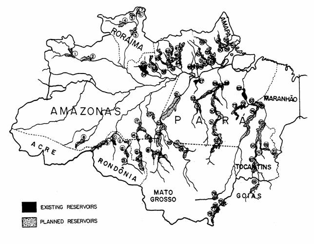
Fig. 3.

Fig. 4

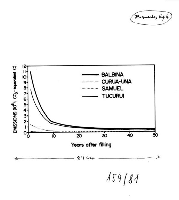
Fig 6